
Output and reproduction scripts
This chapter describes how to export a figure as an image, a video or a Python script. The export controls are below the figure in the main area; only the animation settings are in the "Time" section of the sidebar.
Saving still images
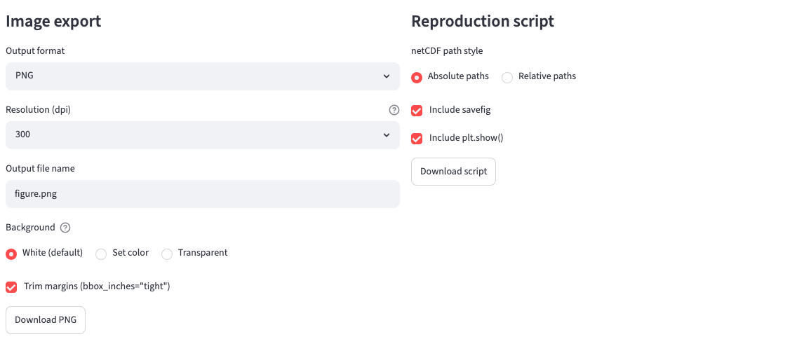
These are the items under "Image export" in the main area.
| Item | Description | Default |
|---|---|---|
| Output format | PNG / JPG / TIFF / SVG / PDF / EPS | PNG |
| Resolution (dpi) | 150 / 300 / 600. In vector formats (SVG / PDF / EPS) it affects only the rasterized elements | 300 |
| Output file name | The extension is replaced to match the output format | figure.png |
| Background | White (default) / Set color / Transparent. The background of the margins outside the plot frame; not reflected in the preview | White |
| Trim margins (bbox_inches="tight") | Trims the margins around the figure | On |
- Save with "Download {fmt}". Multiple panels form one figure, so all panels go into one file.
- JPG is lossy, blurs edges and does not support a transparent background. Use PNG / TIFF / PDF for papers and printing. TIFF is uncompressed and produces large files. EPS may not reproduce transparency and semi-transparent fills exactly, and does not support a transparent background either. Choosing transparent with JPG or EPS outputs a white background.
- The pixel size of the image is the Figure size (inch) × dpi (Basics).
Time-stepping animation
For horizontal maps, vertical cross-sections and 1-D plots, animations are created from "Time" → "Animation" in the sidebar. Time sections are not eligible because time is their axis.
| Item | Description | Default |
|---|---|---|
| Start time / End time | First / last | |
| Step (every n) | 1 to 100 | 1 |
| fps (frames/sec) | 1 to 10 | 4 |
| Resolution (dpi) | Resolution of each frame (50 to 400). Pixels = Figure size × dpi | 100 |
| File format | GIF / MP4. MP4 appears only when ffmpeg is found | GIF |
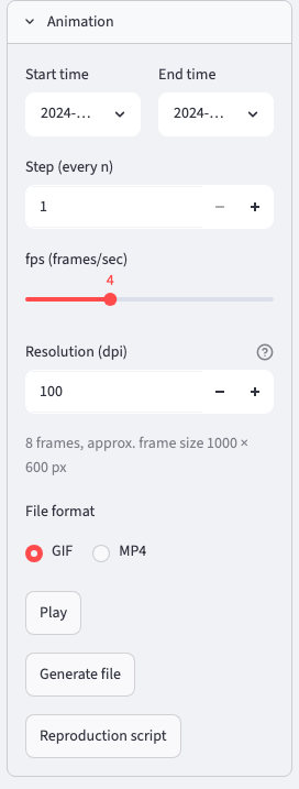
- Below the settings, the number of frames, the approximate frame size and the value ranges within the period ("Value ranges within the time span") are shown. The value ranges are a guide for fixing the minimum and maximum of the fill so that the colors stay consistent between frames.
- "Play" shows the frames in sequence inside the app (drawing time is added, so it can be slower than the fps). "Generate file" creates a GIF or MP4, which you save with "Download animation {fmt}". The file names are animation.gif / animation.mp4. "Reproduction script" creates a Python script that reproduces the animation (Animation reproduction script).
- The whole figure is redrawn for each frame, so the time taken is proportional to the number of frames.
- With multiple panels, the time of all panels advances in sync. Times fixed on the layer side advance as well. Panels whose plot axis is time are drawn as they are, and the "Show time" label follows each frame.
- MP4 uses H.264 and rounds the pixel width and height to even numbers. For installing ffmpeg see Install. GIF concatenates the frames as images and trims the margins when there is no rotation.
Globe rotation animation
"Motion" appears only when the projection is Orthographic and the figure has a single panel.
- "Motion" offers three choices: "Time stepping", "Globe rotation (fixed time)" and "Time stepping + rotation". For data without a time dimension (climatologies, etc.) only rotation is available.
- The start point is the central longitude and latitude of "Projection & region" (the still figure is the first frame). "Add waypoint" places zero or more waypoints (longitude, latitude), and the path ends at "End point lon / lat" (default: the start longitude + 90°).
- The path is a linear interpolation in longitude and latitude, and the longitude turns in the shorter direction. To keep rotating in the same direction, place waypoints less than 180° apart. Frames are distributed among the segments in proportion to their angular distance, so the speed along the path is constant.
- For rotation only, enter "Total frames" (2 to 1000, default 36). For time stepping + rotation, "Frames per time step" (default 1) sets how many frames each time is held, and the total number of frames is the number of times × frames per step. Increasing the count makes the rotation smoother relative to the advance of time.
- A rotating GIF is saved at a fixed size without trimming the margins (the lat/lon labels move from frame to frame, which would make the bounding box jitter).
- As a guide, at 100 dpi one frame takes 0.4 to 0.9 s, and 180 frames take a few minutes. At certain centers cartopy can fail to draw the gridlines; the failed frame and its center are then shown. Change the waypoints or the number of frames, or turn off the gridlines.
Reproduction script
Design
The reproduction script is self-contained Python code that depends only on xarray, numpy, matplotlib and cartopy, so it can be run and edited in an environment without ClimCanvas. The figure drawn inside the app and the figure drawn by the generated script are tested to produce identical images in the same environment. The exception is external colormaps: only when a colormap from cmocean / cmcrameri / cmaps is used does the script import that package.
Structure of the generated script
Under "Reproduction script" in the main area, choose the "netCDF path style" (Absolute paths / Relative paths), "Include savefig" and "Include plt.show()" (both on by default), and save with "Download script". The file name is the output file name with its extension changed to .py. The content can be inspected with "Show generated script" directly below the figure. Relative paths are relative to the directory where the app was started.
The script is laid out from top to bottom in this order.
- A one-line description (the version of ClimCanvas that generated it).
- Only the imports needed (matplotlib, numpy, xarray, cartopy, etc.).
- Imports of external colormaps, registration of custom colormaps and embedded functions (only when needed).
- Data loading such as
ds0 = xr.open_dataset(...). Calendar conversion, attaching coordinate files and dimension name alignment are written out with the same content. - Creation of the Figure, the axes and layer drawing of each panel, colorbars and annotations.
fig.savefig(...)andplt.show(). The savefig arguments carry over the format, resolution, background and margin settings of "Image export" as they are.
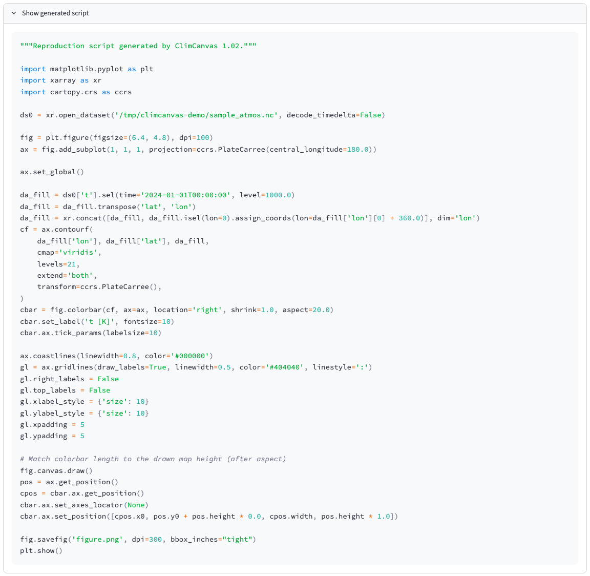
Running it creates the figure file in the same directory. The drawing of each panel is an independent block, so blocks can be deleted or copied as units. Typical places to edit by hand are the data path, the savefig output name and dpi, figsize and the arguments of each drawing call.
When running on another machine
Fonts depend on the environment; if the same font is not available, matplotlib falls back to its default. The 1:50m / 1:10m geographic data are downloaded by cartopy on first use. Reading netCDF requires an xarray backend such as netCDF4.
External and custom colormaps
- When an external colormap (cmocean / cmcrameri / cmaps) is used, the corresponding import (and, for cmaps, a registration line) is added automatically at the top. The same package must be installed in the environment where the script runs.
- Custom colormaps placed in
~/.climcanvas/cmaps/are embedded in the script with their RGB values and registered there. There is no need to copy the colormap files when handing the script to another machine.
Animation reproduction script
"Animation" → "Reproduction script" → "Download animation reproduction script" saves animation.py. It wraps the drawing body in a loop over frames, with the list of times (for rotation, the list of central longitudes and latitudes) written as literals. GIF uses Pillow and MP4 uses ffmpeg, so these must be available in the environment. The netCDF paths are always absolute.
Sessions
Saving and restoring are described in Basics, and the directories where sessions are stored in Usage. This section summarizes the contents and caveats.
- A session JSON is a list of the settings on the screen and includes the paths of the loaded files and of the coordinate files. It does not contain the data itself. If the original files are moved or deleted, restoring fails.
- The display language is not part of the session. Loading a session does not change the language.
- Session file names are free. A downloaded file can be renamed as you like, and saving under a name appends .json to the name you enter. Either can be restored under any name.
- Trying to restore a JSON that is not a session (such as a preset) shows "This does not look like a session JSON".
- When settings change in a newer version, some items of an old session are ignored (without an error). The format of older versions that stored options by display name is converted automatically when loaded.
Presets
A preset stores your preferred data-independent settings in ~/.climcanvas/preset.json and applies them automatically at the next startup. Save and delete under "Save" → "Preset" in the sidebar (Basics).
- The settings on the screen are stored item by item as they are and restored to the same items at startup. Only the settings in the table below are stored.
- Panel and layer settings are stored per panel number (in order of creation), plot mode and layer number (in order of addition), and after startup they are applied only to the panel and layer with the same number. Arrange the appearance on the first panel, save it as a preset, and duplicate the panel when adding more to reuse it.
- Not included: file paths, plot mode, projection and region, fixed dimensions, variable selection, value range and level specification, value transforms, the text of titles, axis labels and colorbar labels, panel labels, text and markers. The appearance of layer kinds not in the table (lines and bars of 1-D plots, the color, width and size of points in scatter mode, etc.) is not included either.
| Location | Settings stored |
|---|---|
| "言語 / Language" at the top of the sidebar | Display language |
| Figure-wide format → Font | Whether to set a font, how to choose, the font |
| "Image export" below the figure | Output format, resolution (dpi), output file name, background (white / set color / transparent) and background color, trim margins |
| "Reproduction script" below the figure | netCDF path style, include savefig, include plt.show() |
| Map & gridlines → Map settings (horizontal map) | Coastlines (show, width, color), country borders, land (fill, color, draw above data), ocean (fill, color), figure frame width |
| Map & gridlines → Gridlines (lat/lon) | Show, lines (show, width, color, style), longitude and latitude intervals, labels (show, sides, longitude labels along the circle and at the pole, latitude label edge, interval, start, rotation, font size, padding) |
| Map & gridlines → Tick marks | Show, longitude and latitude intervals, length, width, orientation, sides, short ticks (add, interval, length, width) |
| Frame | Top/bottom/left/right edges, edge width, edge color |
| Font sizes | Title font size (Text & markers → Title), axis label font size (Labels), tick label font size (Ticks) |
| Show time | Show the time above the plot, position, time format |
| Animation | fps, resolution (dpi), file format |
| Colormap (fill, contours, vectors, streamlines, scatter (points), track, hexbin, 2-D histogram, bubble chart, heatmap) | Colormap group and name, reverse colormap, number of color levels, extend (out-of-range handling). Heatmap: colormap only |
| Colorbar (layers with a colorbar) | Show, position, ticks and label on the opposite side, length, thickness, edge and tick mark widths, gap from the plot, label and tick label font sizes and paddings (the label text is not included) |
| Contours | Line coloring, line color, line width, line styles (positive / negative values), contour labels (show, font size, format) |
| Hatch | Hatch pattern, density, line width, line color, lower and upper bounds |
| Vectors | Coloring and color, grid cells to skip, hide arrows at or below a magnitude threshold (and the threshold), automatic scale and reference vector length, line width, head length, edges (show, color, width), vector key (show, length, label position, font size, position) |
Checks before submitting a paper
ClimCanvas is a tool that draws what it is told to, and it is the user's responsibility to confirm that a figure shows what was intended. Before using a figure in a paper or report, we recommend checking the following four points. The numerical assumptions (selection, subsetting, averaging, missing values, definitions of statistics) are summarized in Computational conventions.
- Read the box "Processing applied to this figure" below the figure and the data section of the reproduction script. The box lists, per panel and only when used, the value transforms (scale a and offset b per variable, with the variable's units attribute), range means (dimension, range, arithmetic or cos(lat)-weighted, number of grid points included, number of missing values within the range), mask-out thresholds, and that vector components are not rotated on a 2-D coordinate grid. It also reports when the main quantity has a value transform that is not applied to the error quantity (also when the units attributes of the error variable and the main variable differ), and when quantities with different units attributes or value transforms are overlaid on the same y-axis of a 1-D plot (the secondary axis and the x-axis of horizontal bars are treated separately). Since units attributes are compared as strings, mere differences in spelling such as "m/s" and "m s-1" are also reported as "may differ". Fixed coordinate values appear verbatim as actual values in
.sel(...), and range means in the.mean(...)line (.weighted(...)when cos-weighted) together with the averaged dimensions (Structure of the generated script). These few lines let you confirm that the level, time, range and weighting are as intended. - Compare the plotted values with your own calculation. If you
printthe array passed to the drawing call in the reproduction script or write it out withto_netcdf, you can compare it with values obtained with GrADS, CDO or your own scripts. Checking even a single point of a range mean, zonal mean or unit conversion reveals mistakes in selection or weighting. - Record the version you used. The version is written in the first line of the reproduction script. Keep a note of which version was used to make the figure. When citing in a paper, cite with the version. How to use the DOIs (the concept DOI shared by all versions and the version DOIs of milestone versions) and citation examples are in Install: citation.
- Check the known bugs. Bugs that affect the plotted values are listed in
KNOWN_ISSUES.mdin the repository together with the affected versions and features. Check before submission, and when a fixed version is released after publication, whether your version and the features you used are affected.
Do not rely too much on the box 'Processing applied to this figure'
The box is an aid for preventing mistakes. It cannot find every mistake. An empty box is no guarantee that the figure is correct. For example, units are compared only as strings of the units attribute, so the same unit written differently (m/s and m s-1) is also reported as "may differ". Conversely, for data without a units attribute, or for combinations outside the check such as several layers of 1-D aggregation or scatter plots, nothing is shown even when the units disagree. Do not rely on the box alone; verify the plotted values yourself as in point 2 above.