
Basic operation
This chapter covers everything from launching the app and loading files to the settings that affect the whole figure. Settings per plot mode are in Plot modes, and layer settings are in Layers: maps and sections and Layers: 1-D, scatter and aggregation.
Launch and quit
ClimCanvas is an app written in Python; it uses the web UI framework Streamlit to display its interface (installed together with the other dependencies). "Launching" means running streamlit run app.py in a terminal, which starts a small web server dedicated to ClimCanvas on that machine. The interface opens in a browser, but it is not a site on the internet: the browser is only connected to the ClimCanvas running on that machine. Both file loading and figure rendering happen on the machine that runs the app.
Activate the Python environment with the dependencies installed (Install 1.3), then run streamlit run in the installation directory. The browser opens automatically; if it does not, open the URL printed in the terminal (usually http://localhost:8501). To quit, press Ctrl+C in the terminal.
Quitting discards your work
The loaded files and settings exist only inside the app process. Reloading the browser or quitting the app returns everything to the initial state, so save a session for any work you want to continue.
On the first launch, a Streamlit card titled "Help agents write better apps" may appear at the top right. It is not a ClimCanvas feature and can be closed (FAQ).
ClimCanvas itself sends nothing over the network. There are two exceptions: cartopy automatically downloads Natural Earth data such as coastlines the first time a given scale is used (Plot modes), and Streamlit, which displays the interface, sends anonymous usage statistics to its developers by default. To stop the latter, write the following in ~/.streamlit/config.toml on the machine that runs the app (Install 4.3).
Procedures for each way of operating (running on your own PC, running on a lab server and using it via SSH, several people connecting to one machine in a class) are in Usage. The configuration file config.toml lets you restrict the directories that can be opened and change where sessions are saved.
UI language
Select the display language with "言語 / Language" at the very top of the sidebar (日本語 / English / 简体中文 / 한국어). The language is not saved in sessions. To keep the same language from the next launch on, save it in a preset.
Turn off automatic browser translation
When automatic translation in Chrome or similar browsers kicks in, the on-screen text is replaced without warning, and the display may break (for example, buttons stop working). Set localhost to "never translate this site". To change the display language, use the language setting inside the app. See the FAQ for details.
Screen layout
The screen is divided into the sidebar on the left and the main area on the right. All settings are made in the sidebar; the main area holds the results and the output. "About" in the "⋮" menu at the top right shows the version in use and links to the feedback form and to bug reports (GitHub Issues) (FAQ).
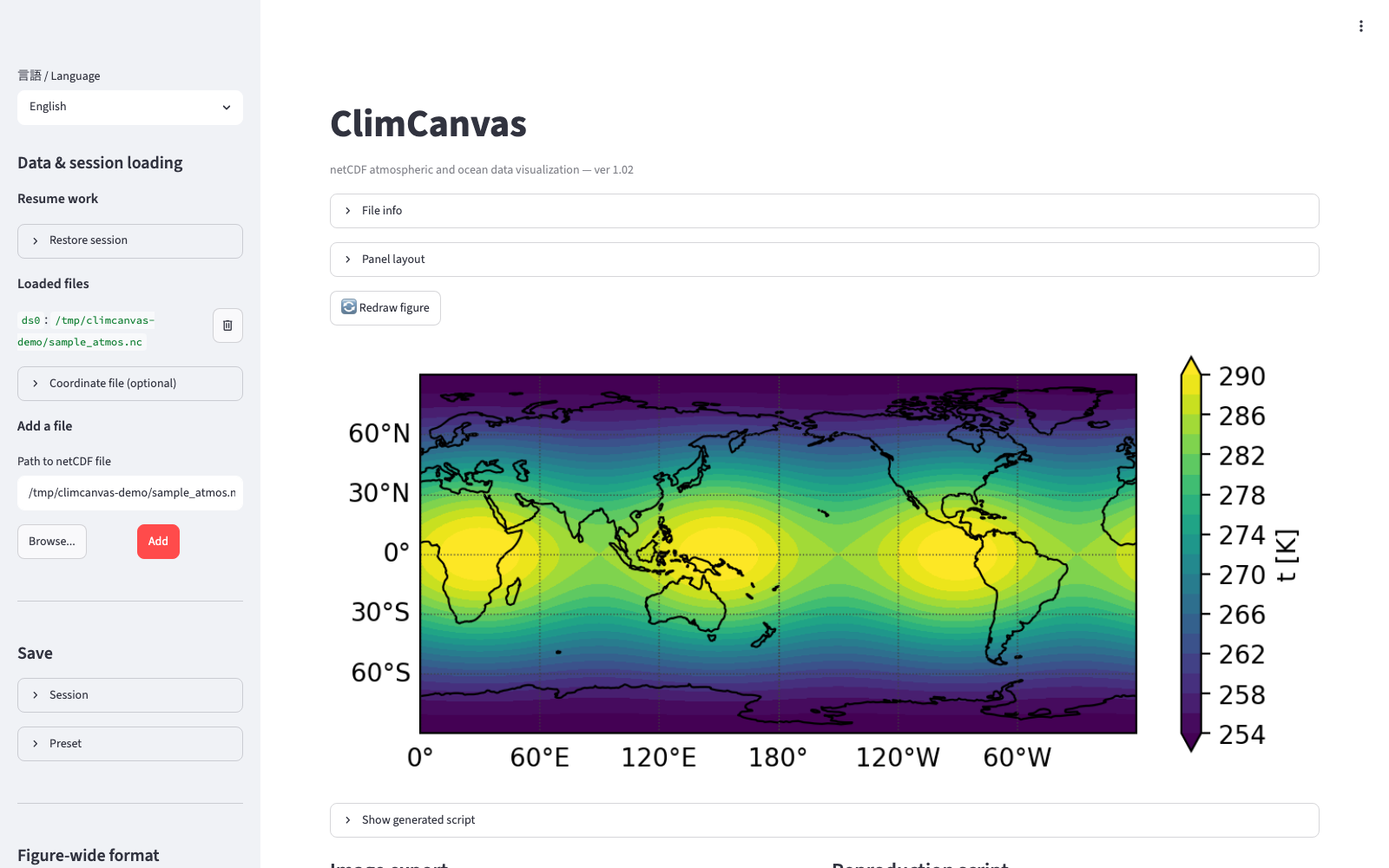
| Main area (from the top) | Contents |
|---|---|
| File info | List of the variables and coordinates of the loaded files and the result of coordinate-role auto-detection (details) |
| Panel layout | Number of rows and columns of the figure, adding, duplicating and deleting panels, selecting the panel to edit (Multiple panels) |
| Redraw figure | Button that redraws the figure with the current settings. Press it when a change did not show up in the figure (for example, you forgot to press Enter in a number field). Do not reload the browser: that clears every setting |
| Figure | The rendered result |
| Processing applied to this figure | Shown in a box below the figure only when applicable: value transforms (factor a, offset b and the variable's units attribute), range means (dimension, range, method, number of grid points, number of missing values within the range), mask-out thresholds, how vectors on a 2-D coordinate grid are treated, that value transforms are not applied to error quantities, and that quantities with different units or value transforms share the same axis in a 1-D plot. Use it to confirm that the units, ranges and weights are the ones you intended. It is a help against mistakes, not a detector of every mistake, so do not rely on it alone and check for yourself (Checks before submitting a paper) |
| Image export / Reproduction script | Saving the image (format, resolution, background) and downloading a Python script that reproduces the figure (Output and reproduction scripts) |
| Show generated script | Inspect the contents of the reproduction script |
The figure is redrawn every time a setting changes. With heavy data, it is more comfortable to narrow the region and the time first and adjust the fine formatting afterwards (Performance guide).
Order of the sidebar sections
The sidebar is arranged from the top in the following order. The first half holds settings that affect the whole figure; the second half holds the settings of the panel selected as "Panel to edit".
| Section | Contents |
|---|---|
| 言語 / Language | Display language |
| Data & session loading | Resuming work (restoring a session), loaded files, new work / adding files |
| Save | Session, preset (Saving) |
| Figure-wide format | Figure size, font, layout adjustment (margins), shared colorbar (all panels) (Figure-wide format) |
| Plot mode (per panel) | Plot mode of the panel being edited (Plot modes) |
| Mode-specific sections | See the table below |
| Plot size | Aspect ratio of the plot area (axes box) (Figure size and aspect ratio) |
| Text & markers | Title, panel label, text, markers (Text and markers) |
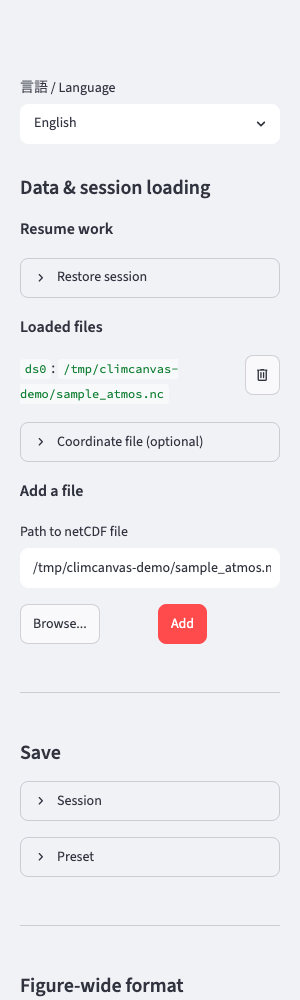
The mode-specific sections depend on the plot mode.
| Plot mode | Order of sections |
|---|---|
| Horizontal map | Projection & region → Time → Layers → Map & gridlines |
| Vertical cross-section | Cross-section → Time → Layers → Axes & labels → Frame & background |
| Time section | Time section type → Layers → Axes & labels → Frame & background |
| 1-D plot | Plot axis → Time (when the x-axis is not time) → Layers → Axes, labels & legend → Frame & background |
| 1-D plot (aggregation) | Layers → Axes, labels & legend → Frame & background |
| 2-D plot | Plot variables → Layers → Axes, labels & legend → Frame & background (for the heatmap: no layers, and Axes & labels) |
| 2-D plot (aggregation) | Plot variables → Layers → Axes & labels → Frame & background |
In the "Time" section you also pick the values of other dimensions that need fixing (such as vertical levels). See Data handling.
Loading files
Specify a netCDF file under "Data & session loading" → "New work" in the sidebar.
- Enter the path in "Path to netCDF file" and press "Add".
- Pressing "Browse..." opens the file dialog of the OS. The dialog opens on the machine that runs the app, so use it when the app runs on your own PC.
- When
allowed_dirs(restriction of the directories that can be opened) is set in the configuration file, "📁 Choose from allowed directories" appears instead of "Browse...", and you can walk through the folders to pick a file. A path outside the allowed directories gives an error.
Loading is lazy. Only the metadata and coordinates are read when a file is opened, so even a file of tens of GB opens instantly.
Multiple files
Once the first file is loaded, a list appears under "Loaded files", and "Add a file" adds the second and later files in the same way. Files get the IDs ds0, ds1, … in the order they were loaded, and each layer can choose which file's variable to plot (for example, overlaying reanalysis winds with sea surface temperature from another file).
- "Delete" in the list removes a file. The IDs are renumbered over the remaining files.
- Dimension names such as latitude and longitude are aligned automatically even when they differ between files (
latandlatitude, etc.). Overlaying files whose coordinate values do not match on the same axes gives an error when rendering.
Data whose longitude and latitude are in separate files
Regional-model output whose longitude and latitude are 2-D variables in separate files such as FLON.nc / FLAT.nc is attached under "Coordinate file (optional)" below each file in "Loaded files". Specify the longitude file and the latitude file (only the longitude side if they are in the same file) and press "Apply": the longitude and latitude are attached as coordinates, and horizontal maps become available. "Detach" removes them.
- Files are chosen the same way as the main file (entering a path, "Browse...", "Choose from allowed directories").
- For the second and later files (terrain height, surface pressure, etc.) a checkbox "Use the same coordinate files as ds0 (FLON.nc, FLAT.nc)" appears. Tick it to attach the same coordinate files as the first file (this is not done automatically; if the grids differ, attaching stops with an error).
- The specification is saved in the session, and the reproduction script opens the same files.
- A Lambert conformal conic grid is recognized automatically from the longitude and latitude and becomes the initial projection (Data handling).
File info
Opening "File info" in the main area shows the following for each file. It is the information you would see with ncdump -h, plus the result of the coordinate-role detection.
| Item | Contents |
|---|---|
| ID and path | The ID such as ds0 and the loaded path |
| Data variables | Table of variable name, dimensions, shape, units and long_name. Coordinate variables are not included |
| Coordinate variables | Table of coordinate name, dimensions, length, range and units |
| Dims without coordinate variables (bare dims) | Dimensions without coordinate values. Handled by the indices 0, 1, 2, … |
| Auto-detected coordinates (ds0) | Which coordinate was assigned to each of the latitude / longitude / vertical / time roles. A role that could not be detected is "(none)", and the plot modes that use that role do not appear among the choices |
| Dimension to treat as time | Manual override of the auto-detection (Data handling) |
The rules for detecting coordinate roles are in Data handling.
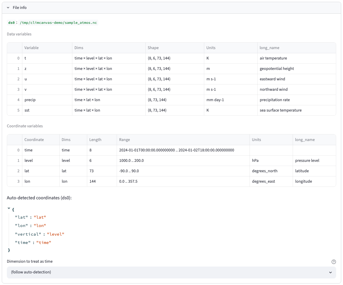
Figure size and aspect ratio
"Figure-wide format" → "Figure size" sets the size of the whole figure (the matplotlib figure) in inches. Even with multiple panels there is one setting for the whole figure.
| Aspect ratio | Width × height |
|---|---|
| 6.4:4.8 (matplotlib default) | 6.4 × 4.8 inch (default) |
| 1:1 | 6.4 × 6.4 |
| √2:1 (A4) | 6.4 × 4.53 |
| 16:9 | 6.4 × 3.6 |
| Custom values | Enter the width and height, 1 to 30 inch |

The pixel size of the saved image is "width × dpi" by "height × dpi" (dpi is "Resolution (dpi)" under "Image export": 150 / 300 / 600, default 300). Because the margins are trimmed when saving, the actual image is slightly smaller.
How the aspect ratio of the plot area (axes) is determined depends on the plot mode.
| Plot mode | What determines the axes aspect ratio | When the figure size changes |
|---|---|---|
| Horizontal map | The projection and region (the map shape is fixed) | The map shape stays the same; the surrounding margins grow or shrink |
| All other modes | The figure size (the plot area fills the figure) | The axes themselves stretch |
Outside horizontal maps, "Plot size" → "Axes box aspect ratio" fixes the height / width ratio of the plot area (0.5 for landscape, 2.0 for portrait). The figure margins are changed under Layout adjustment.
Figure-wide format
Font
Ticking "Figure-wide format" → "Font" → "Set font" applies the same font to all text: title, axes, ticks, colorbar and annotations. When not set, the matplotlib default (DejaVu Sans) is used.
- "How to choose" has two levels. "Common fonts" lists only the well-known fonts that are installed, and "Search all fonts" narrows down every font detected by matplotlib as you type.
- When the title or annotations contain Japanese text, choosing a Japanese font (Hiragino Sans on macOS, Noto Sans CJK JP on Linux, etc.) avoids missing glyphs (□). When the figure contains Japanese or other such characters and the font does not support them, a warning appears before rendering.
Fonts depend on the environment
When the reproduction script runs on another machine without the same font, matplotlib falls back to its default.
Layout adjustment (margins)
"Figure-wide format" → "Layout adjustment (margins)" corresponds to matplotlib's subplots_adjust.
| Item | Contents | Default |
|---|---|---|
| Set gaps between panels | Horizontal (wspace) and vertical (hspace). Ratios to the panel width and height; negative values overlap cells to tighten the layout | 0.2 / 0.2 |
| Set outer figure margins | Left, right, bottom and top in figure coordinates (0 to 1) | 0.125 / 0.9 / 0.11 / 0.88 |
Because the aspect ratio of a horizontal map is fixed, tightening the margins may not bring the maps closer together. In that case, bring the aspect ratio of the figure size closer to the shape of the maps.
Shared colorbar
"Figure-wide format" → "Shared colorbar (all panels)" adds one colorbar shared by all panels. The colors of the first fill layer are used as the representative, so use the same colormap and value range for the fills of all panels. See Multiple panels for details.
Text and markers
"Text & markers" at the end of the sidebar holds the title and annotations of the panel being edited.
Title
Set "Figure title" and "Title font size". An empty title is not shown.
Panel label
Labels such as (a), (b) used in multi-panel figures of papers. Tick "Show panel label" and set "Label text", "x", "y" (relative coordinates with the lower left of the plot frame at 0, 0 and the upper right at 1, 1; the default 0, 1.02 is just outside the upper left), "Font size" (default 12), "Bold" and "Label color". Change the text for each panel.
Text
"Add text" places text at any position. Each press adds an item "Text 1", "Text 2", …, and "Delete this text" removes it.
| Item | Contents |
|---|---|
| Text | The text to show. Hidden when empty |
| Coordinate system of the position | axes (relative position in the plot frame, 0 to 1) or data coordinates |
| x, y | The position. In data coordinates: longitude and latitude on a horizontal map (following the projection), axis values in other modes |
| Horizontal alignment (ha) / Vertical alignment (va) | Which part of the text is placed at x, y |
| Rotation (deg), Font size, Text color | Formatting |
| Add edges | A box around the text. Set its color and width |
Axes coordinates suit fixed labels in a corner of the figure; data coordinates suit annotations of locations on a map (typhoon position, station names, etc.).
Markers
"Add marker" places markers such as ○ ■ ▲ × ◇ ☆ at any position. Set "Marker type", "Size (pt)", "Marker color", "Add edges", and the same "Coordinate system of the position", "x" and "y" as for text.
Saving
"Save" in the sidebar offers two kinds of saving.
| Kind | Contents | Restoring |
|---|---|---|
| Session | Saves the entire state, including file names, variables, times, region and layer setup, as JSON. The blue tab saves under a name on the machine running ClimCanvas ("To this PC" in local operation, "To the server" in remote operation); the orange tab downloads to your own PC | "Data & session loading" → "Resume work" → "Restore session" |
| Preset | Saves only the preferences that do not depend on the data, such as the display language and font, to ~/.climcanvas/preset.json. Applied automatically at the next launch. "Delete startup preset" removes it. The list of saved settings is in Preset |
Automatically at launch |
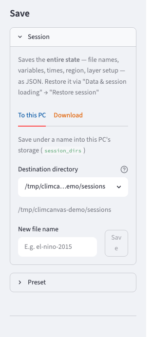
The session JSON contains only the paths of the netCDF files, not the data themselves. Restoring fails if the original files are moved or deleted. For the save directory and the procedure per way of operating, see Usage (local) and Configuration file.
Performance guide
What determines the rendering cost is not the total file size but the number of points in the slice actually drawn.
- Opening a file reads only the metadata and coordinates, so it is instant even for large files. Rendering reads from disk only the one slice obtained by fixing the time and vertical level and cropping the region.
- The main causes of slowness are the number of horizontal grid points after cropping (about a million points of a 0.25° global grid is fine; a wide area of a km-scale grid is sluggish), range means (the whole averaging range is read), animation (proportional to the number of frames), and the number of panels and layers.
- The figure is redrawn from scratch every time a single setting changes. With heavy data, narrow the region and time first and adjust the formatting afterwards.
- Only at the moment you switch the value range to manual, the whole variable is scanned to find the default values. With a huge variable this can take a few seconds.
- Jumping to a specific time depends neither on the number of times nor on their position (the time coordinate is searched in memory, and only the relevant part of the data is read). However, irregular files with many times in one chunk, compressed netCDF, and online-only files such as those in Dropbox take extra time to read.
- Where the number of times matters directly is the time selector. In files with tens of thousands of steps, sending the choices themselves can be the cause of sluggishness.