
Plot modes
This chapter describes the plot mode selected for each panel and the settings specific to each mode. The settings for each layer kind are in Layers: maps and sections and Layers: 1-D, scatter and aggregation, fixing dimensions and ranges are in Data handling, and examples of the figures you can draw are in the Gallery.
Choosing a mode and when each appears
Select it in the sidebar under "Plot mode (per panel)" → "Plot mode". The choices are narrowed by the coordinate roles of the loaded data, and the first one is the default. The conditions are listed in Data handling.
| Plot mode | What it draws |
|---|---|
| Horizontal map | A map on a map projection. Fill, contours, hatch, vectors, streamlines, scatter (points), and tracks are overlaid |
| Vertical cross-section | Longitude–height and latitude–height sections, sections along the great circle between two points, and, for data on a 2-D coordinate grid, sections along a grid row or column, a parallel, or a meridian. Terrain mask |
| Time section | Time–height, time–latitude, and time–longitude sections (Hovmöller diagrams) |
| 1-D plot | Lines, line bundles, filled bands, stack plots, bar charts |
| 1-D plot (aggregation) | Histogram, ECDF, box plot, violin |
| 2-D plot | Scatter, bubble chart, categorical heatmap |
| 2-D plot (aggregation) | 2-D histogram, hexbin |
"Plot size", right after "Plot mode", fixes the aspect ratio of the plot area (the axes box). "Axes box aspect ratio" is 1:1 / 6.4:4.8 (matplotlib default) / "Custom"; the default is 1:1 for the 2-D plot modes and 6.4:4.8 for the others. With "Custom", enter "Height / width" as a number (0.5 for landscape, 2.0 for portrait). This setting is not available for horizontal maps, because the shape of a map is determined by the projection and the display extent.
Horizontal map
Projection and region
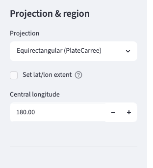
"Projection" offers the following 7 choices. The default is equirectangular (PlateCarree).
| Projection | Specific items |
|---|---|
| Equirectangular (PlateCarree) | Central longitude (with an extent set, the midpoint of the range is used automatically) |
| Robinson projection (Robinson) | Central longitude |
| Equal Earth projection (EqualEarth) | Central longitude |
| Polar stereographic, North Pole (NorthPolarStereo) | The lat/lon extent is always set; "Circular frame" (default on) |
| Polar stereographic, South Pole (SouthPolarStereo) | Same as above |
| Orthographic projection | Central longitude, central latitude (default 20) |
| Lambert conformal conic (LambertConformal) | Central longitude (default 140), central latitude (default 35), standard parallels 1 and 2 (defaults 33 and 45) |
- "Set lat/lon extent" with "Longitude min / max" and "Latitude min / max" determines the display extent. See Data handling for the defaults and the cropping rules.
- The central longitude is 180 (140 for Lambert) when no lat/lon extent is set. When an extent is set in the equirectangular projection, the midpoint of the range is used automatically and no input field appears. In the Robinson and Equal Earth projections, "Match the central longitude to the range midpoint" (default on) follows the midpoint of the range; uncheck it to enter a number (the map curves as the value moves away from the midpoint). In the polar stereographic, orthographic, and Lambert projections the central longitude does not follow changes of the extent, so a warning appears when it is 90° or more away from the midpoint of the range.
- Narrowing the longitude range in a polar stereographic projection gives a sector-shaped map, and the placement of the latitude labels can be chosen from "Inside the map (default)", "Along the frame", and "Hidden".
- For 2-D coordinate data on a Lambert grid, the projection estimated from the grid together with its central longitude and standard parallels are the initial values (Data handling).
Coastlines, borders, land, and geographic data resolution
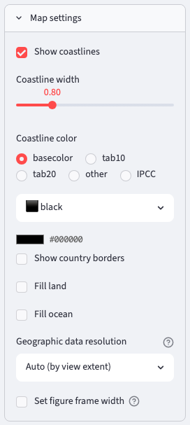
These are the items of "Map settings".
| Item | Content | Default |
|---|---|---|
| Show coastlines | Width (0.2–3.0) and color. Turning it off also removes the country borders | On, 0.8, black |
| Show country borders | Off | |
| Fill land | Land color | Off, #d9d2c2 |
| Draw above data | Hides fill, hatch, and vectors over land behind the land. Contours, streamlines, tracks, coastlines, country borders, lat/lon lines, boxes, annotations, scatter points, and the vector key appear above the land | Off |
| Fill ocean | Ocean color | Off, #cfe2f3 |
| Geographic data resolution | The Natural Earth scale shared by coastlines, country borders, land, and ocean. "Auto" / "Coarse (1:110m)" / "Medium (1:50m)" / "Fine (1:10m)" | "Auto" |
| Set figure frame width | Width of the frame line (0.2–5.0). Also applies to the circular frame of the polar stereographic projections | Off (matplotlib default) |
- Geographic data resolution "Auto" uses 1:50m when the shorter side of the display extent is 50° or less, 1:10m when it is 15° or less, and 1:110m otherwise. The 1:50m and 1:10m data are downloaded automatically by cartopy on first use (an internet connection is required).
- "Draw above data" can cover the spill of data over land, as with sea surface temperature where the land cells also hold values. The extent of the land fill is determined by the Natural Earth land polygons and is unrelated to the missing values of the data.
Gridlines and labels
"Gridlines (lat/lon)" → "Show lat/lon lines & labels" (default on) is the parent switch; the lines and the labels can be toggled independently. The "no lines, labels only" style common in journal figures is also possible.
| Item | Content | Default |
|---|---|---|
| Show lines | Width (0.1–2.0), color, line style (dotted / solid / dashed) | On, 0.5, gray, dotted |
| Meridian interval / Parallel interval | Degrees. 0 for automatic | 0 |
| Show labels | The sides on which to show labels (Left / Right / Top / Bottom) | On, left and bottom |
| Label longitude interval / Label latitude interval | Can differ from the line interval (lines every 10°, labels every 30°, etc.). 0 for the same as the lines | 0 |
| Label start longitude / Label start latitude | Labels are placed every interval starting from this value (start 15°, interval 30° gives 15, 45, 75, …). 0 for multiples of the interval | 0 |
| Longitude label rotation (deg) | 0 | |
| Set latitude label rotation | Off for automatic (in the polar stereographic projections, along the edge or the meridians). On to fix the angle | Off |
| Label font size / Label padding (pt) | 10 / 5 |
Automatic thinning of labels
When labels overlap, cartopy automatically thins out the overlapping ones (every other label appears to be shown with an interval of 20°, etc.). There is no setting to disable this. Rotating the longitude labels (around 45°), reducing the font size, or widening the figure shows them all.
In the polar stereographic projections, in addition to "Sides to show longitude labels on" (Top / Bottom), you specify "Longitude labels along the circle", "Longitude label at the pole" (for a sector-shaped map), and "Latitude labels" ("Inside the map (default)" / "Along the frame" / "Hidden"; with "Along the frame", "Edges to show" is "Both" / "Left only" / "Right only").
Tick marks and boxes
"Tick marks" are drawn only in the equirectangular projection. Turn on "Show tick marks" (default off) and specify the longitude interval (default 30), the latitude interval (default 15), the length (default 4), the width (default 0.8), the orientation ("Outside" / "Inside" / "Both"), and the sides to draw them on (default left and bottom). "Add short ticks (minor ticks)" inserts shorter ticks at a finer interval between the long ones (long every 10° plus short every 5°, etc.; short ticks at the same positions as long ones are removed automatically, so they alternate). No labels are attached.
"Boxes (rectangular region outlines)" → "Add box" draws the outline of a rectangle given in longitude and latitude on the map. Specify "Longitude min" / "Longitude max", "Latitude min" / "Latitude max", "Line color" (default red), "Line width" (default 1.5), and "Line style". When the longitude max is smaller than the min, the rectangle crosses the date line.
Section paths
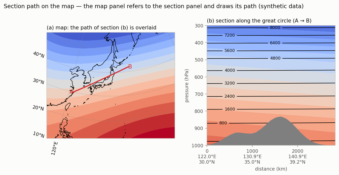
When a multi-panel figure contains a vertical section panel (Vertical cross-section), "Section paths" overlays the path of the vertical section panel (Vertical cross-section) on the map as a line. The vertical section panels that have been set up appear under "Section panels to overlay" as "Panel 2" and so on; select them (when there are none, only a note to that effect is shown). Specify the line color (default red), width, and line style, and the end-point labels (default on; the start and end labels of each section can be written freely, and an end left blank gets no label). The path is derived from the settings of the section panel every time the figure is drawn, so the line follows when you move the section. The kind of path (parallel or meridian, grid row or column of the data, great circle) does not matter.
Map aspect ratio
The aspect ratio of a cartopy map is determined by the projection and the display extent and does not change with the figure size. In the equirectangular projection it is longitude span : latitude span (2:1 for the globe), the Robinson projection is about 2:1, the circular frame of the polar stereographic projections and the orthographic projection are 1:1, and the Lambert projection depends on the central latitude, the standard parallels, and the extent. If the figure is wider than the map, white space appears on the left and right; if it is taller, above and below. For a global equirectangular map, a width of 10 and a height of 5.5 inches is a good starting point. For how to handle wide gaps between rows in multi-panel figures, see Multiple panels and Layout adjustment.
Vertical cross-section
- Select the kind of section under "Cross-section" → "Orientation". The choices depend on the data grid.
- Data with 1-D longitude and latitude: "Longitude-height (fix latitude)", "Latitude-height (fix longitude)", "along the great circle between two points (distance–height, interpolated)".
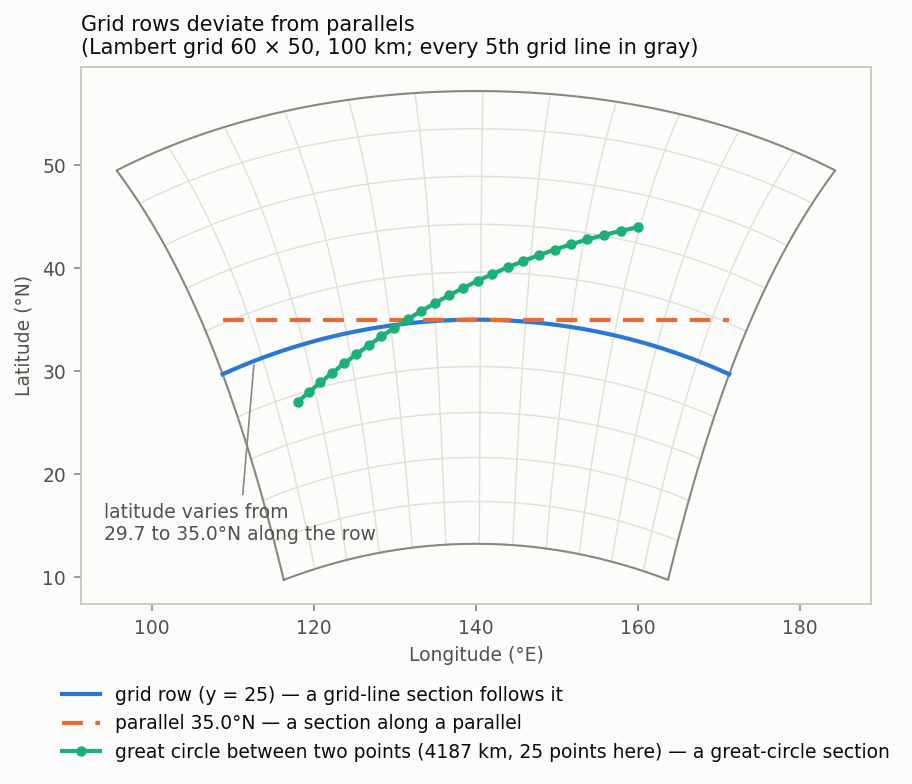
- Data with 2-D longitude and latitude (2-D coordinates): "along a grid row (x–height, row fixed)", "along a grid column (y–height, column fixed)", "along a parallel (longitude–height, interpolated)", "along a meridian (latitude–height, interpolated)", "along the great circle between two points (distance–height, interpolated)".
- The fixed latitude or longitude (the grid row or column for 2-D coordinates) is specified per layer under "Layers"; for latitude and longitude, a range mean can be chosen instead of a fixed value. With 2-D coordinates, fixing a grid row or column displays the latitude and longitude range of that row or column (because, as the figure below shows, a grid row deviates from a parallel).
- The orientations marked "interpolated" place points along the path at roughly the grid spacing and bilinearly interpolate the value at each point from the 4 surrounding grid points. For a parallel, enter the latitude and the start and end longitudes; for a meridian, the longitude and the start and end latitudes; for a great circle, the longitude and latitude of the start and end points. Uncheck "Automatic number of points (spacing ≈ grid spacing)" to specify the number of points. The path length, the number of points, the point spacing, the grid spacing, and the part of the path that lies inside the grid are displayed. Points outside the grid become missing. The interpolation is reported in the box "Processing applied to this figure" below the figure. For the details of the interpolation (how the points are placed, how the grid indices are found, the weights, and the rules for missing values), see Interpolation of sections along a path.
- The sliders "Height / pressure level range" and "Longitude range" ("Latitude range", or "Grid index range" for a grid row or column) narrow the drawn range. For a section along a path, the x-axis range is determined by the path.
- "Label ticks with longitude and latitude" (shown for grid row/column and great-circle sections, default on) shows, at each x tick, the axis value (grid index or distance in km) and the longitude and latitude of that position on three lines.
- The available layers are fill, contours, hatch, vectors, and streamlines. In great-circle and grid row/column sections, the vector and streamline components are drawn as the chosen variables and are not projected onto the direction of the section (a note appears in the frame).
- "Axes & labels" → "Axes" has "Invert x-axis", "Invert y-axis" (default on for a pressure axis), "Show y-axis on the right", "Use log scale on the y-axis", and, when the x-axis is longitude, "Show x-axis (longitude) as °E / °W". "Labels" and "Ticks" are the same as in Axes, legend and frame.
- "Frame & background" → "Frame" has only "Set edge width".
In a multi-panel figure, the section path can be overlaid as a line on a horizontal map panel (Section paths).
Terrain mask
The area below the ground can be masked. Turn on "Terrain mask" → "Cover the area below the ground with terrain": every layer is drawn with the data as they are, and then a filled polygon covering the area below the ground is overlaid to hide it (the values below the ground are not turned into missing values; with an automatic color range, the values below the ground enter the range, so a note appears in the frame).
"How the ground is determined" is narrowed by the units of the vertical coordinate. The variable is selected from all loaded files with its units, as in "ds1: ps [Pa]", and the variables whose units can be converted come first (Pa and hPa, m and km; geopotential in m2 s-2 is divided by g to give m). When the surface pressure or terrain height is in a separate file, add that file and select it (for a section along a path, that file also needs coordinate files).
| How the ground is determined | Vertical coordinate | Variables used |
|---|---|---|
| Surface pressure variable | Pressure | Surface pressure (horizontal 2-D) |
| Terrain height variable | Height | Terrain height (horizontal 2-D) |
| Height variable and terrain height variable | Pressure | A height variable (geopotential height, etc.) and the terrain height. In each column, the pressure at which the height equals the terrain height is found |
"Height variable and terrain height variable" derives the surface pressure, when no surface pressure variable is available, from the height field on pressure levels (Z, etc.: a variable with a vertical dimension and units of m / km / gpm / m2 s-2) and the terrain height (horizontal 2-D, m / km). In each column of the section, the height and the terrain height are brought to m, and the pressure is interpolated linearly in log p between the two adjacent pressure levels that bracket the terrain height (for example, with a terrain height of 1500 m, Z(850 hPa) = 1450 m, and Z(800 hPa) = 1950 m, the ground is at about 845 hPa). In columns where the terrain height is below the height of the lowest level (over the ocean, etc.), the ground lies below the data, so nothing is drawn. If the model provides a surface pressure variable, using it is more direct.
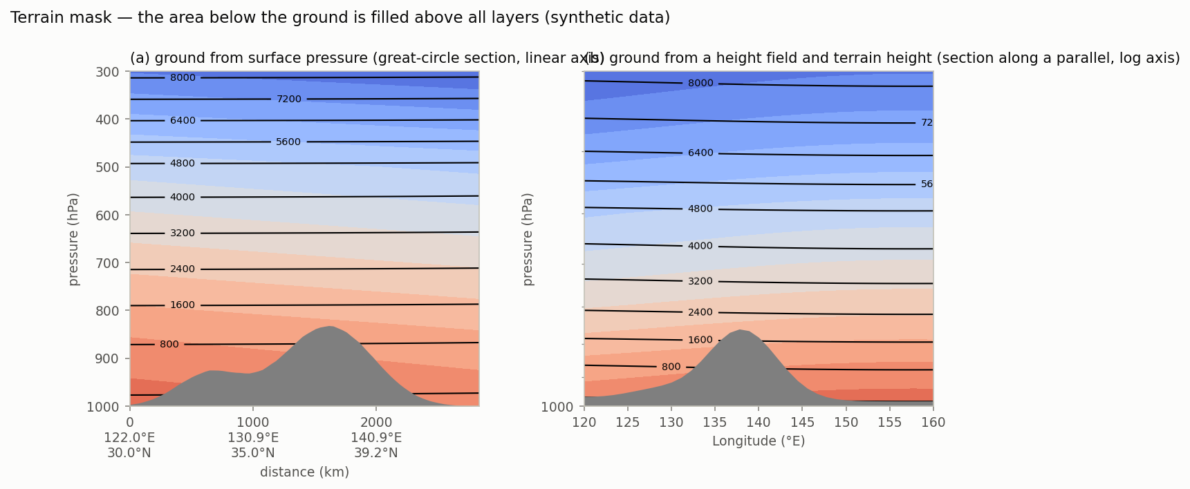
Time section
- "Kind" offers "Time-height", "Time-latitude", and "Time-longitude"; only those supported by the roles of the data appear. Time-height has time on the x-axis; time-latitude and time-longitude follow the Hovmöller convention with time on the y-axis (running downward).
- The "Time range" slider narrows the period.
- The dimensions not used by the section are fixed per layer; for the latitude and longitude directions, a range mean can be chosen as well (the vertical direction accepts a fixed value only).
- Vectors and streamlines are not available (two components cannot be defined on a time axis).
- When the time axis is of datetime type, "Time axis format" appears under "Axes". On a numeric time axis (integer years or a 360-day calendar), manual tick positions can be used instead of the format.
1-D plot
- Select the dimension for the x-axis under "Plot axis" → "Axes" (any dimension that has a coordinate variable). The "Range" slider and input fields narrow the range (Data handling). When the x-axis is longitude, "Unwrap x-axis cyclically (display beyond 360°)" appears.
- The available layers are line, line bundle, line fill, stack plot, and bar chart. The dimensions other than the x-axis are fixed or range-averaged per layer.
- When the panel has a bar chart layer, "Bar placement" ("Overlap" / "Side by side" / "Stacked") appears. With "Side by side", "Gap between bars" (default 0.05) is also specified.
- "Axes, labels & legend" contains "Axes", "Labels", "Secondary axis (right)", "Ticks", and "Legend". The default x-axis label is "dimension name [units]".
- "Secondary axis (right)" is created only when "Draw on the secondary (right) axis" is turned on in a layer. Besides the label, log scale, inversion, manual range, tick positions, and gridlines, "Align a value across both axes" widens the ranges so that a value such as 0 sits at the same height on the left and right axes.
1-D plot (aggregation)
Under "Plot type", select "Histogram / ECDF" (x = value, y = count or fraction) or "Box / violin" (x = the series side by side, y = value; one layer is one series). For box / violin, "Orientation" ("Vertical" / "Horizontal") can also be chosen; with "Horizontal", the series names go on the y-axis and the values on the x-axis.
- The candidate variables are the numeric variables that do not have latitude or longitude as a dimension. Time is used as the dimension to aggregate, so there is no "Time" section and no animation.
- The available layers are histogram, ECDF, and line for "Histogram / ECDF", and box plot and violin for "Box / violin".
- When the axis labels are left empty, x gets the "variable name [units]" of the first layer and y gets count / probability density, etc., automatically. The range and label of "Secondary axis (right)" can also be specified.
2-D plot
Under "Plot variables" → "Plot type", select "Scatter / bubble" or "categorical heatmap". There is no "Time" section and no animation.
For scatter / bubble, select "x-axis variable", "y-axis variable", and, for the size of the bubbles in a bubble chart, "z-axis variable (for bubble chart, optional)". x and y are shared by all layers in the panel, while the dimension to plot and the dimensions to fix are specified per layer. The available layers are scatter and bubble chart. The default "Plot size" is 1:1.
categorical heatmap
Shows one 2-D variable as a matrix of equal-width colored cells. It cannot be used with latitude/longitude data (use the fill of a horizontal map instead). It has no layers and is drawn from the panel settings alone.
| Item | Content | Default |
|---|---|---|
| Variable, x-axis dim, y-axis dim | Extra dimensions are fixed with "Fix: {dim}" (by index when there is no coordinate) | |
| Colormap, Reverse colormap | ||
| Use equally spaced levels | When on, "Automatic value range" (when off, "Min" and "Max") and "Number of color levels" (3–60). When off, enter the boundary values directly in "Levels (comma-separated)" (unequal spacing allowed) | On, 21 |
| extend (out-of-range handling) | both / neither / min / max | both |
| White near zero | Makes the color band containing 0 white | Off |
| Square cells (aspect=equal) | Off | |
| Show values in cells | "Number format" (default %.2g), "Annotation font size", "Annotation text color" | Off |
| Colorbar | The same items as a fill layer (Layers: maps and sections) | Shown |
Row 0 comes at the top. To change the row direction, use "Axes & labels" → "Axes" → "Invert y-axis". The coordinate values become the tick labels, and a dimension without coordinates gets indices. "x tick label rotation (deg)" and "y tick label rotation (deg)" under "Ticks" apply to the category labels. The value transform and mask-out items are also at the end.
2-D plot (aggregation)
Under "Plot variables", select "x-axis variable" and "y-axis variable" (the candidates are the numeric variables that do not have latitude or longitude as a dimension); all pairs of samples of the two variables are aggregated. The available layers are 2-D histogram and hexbin. The colors are shown by a colorbar, so there is no legend. When the axis labels are left empty, "variable name [units]" is filled in automatically. The default "Plot size" is 1:1.