
Interpolation of sections along a path
When you choose an "Orientation" of the vertical cross-section marked "interpolated" (along a parallel, along a meridian, along the great circle between two points), ClimCanvas does not simply line up grid-point values: it takes points on the path and bilinearly interpolates the value at each point from the surrounding grid points. This chapter explains what that interpolation actually does. It focuses on grids whose longitude and latitude are 2-D (2-D coordinates: the Lambert grid of a regional model, WRF, ocean-model grids, and so on), but the "along the great circle between two points" section on an ordinary grid with 1-D longitude/latitude uses the same mechanism. Because interpolation changes the values, its use is always reported in the box "Processing applied to this figure" below the figure.
Why interpolation is needed
On a grid with 2-D longitude/latitude, the grid rows and columns do not coincide with parallels and meridians. For example, on the ClimCORE Lambert grid (817 × 661, 5 km), latitude changes by about 5°, from 30.3°N to 35.2°N, along a single row, and longitude changes by nearly 10° along a single column. A section "along a grid row" has exact values without interpolation, but it is no substitute for "the section at 35°N".
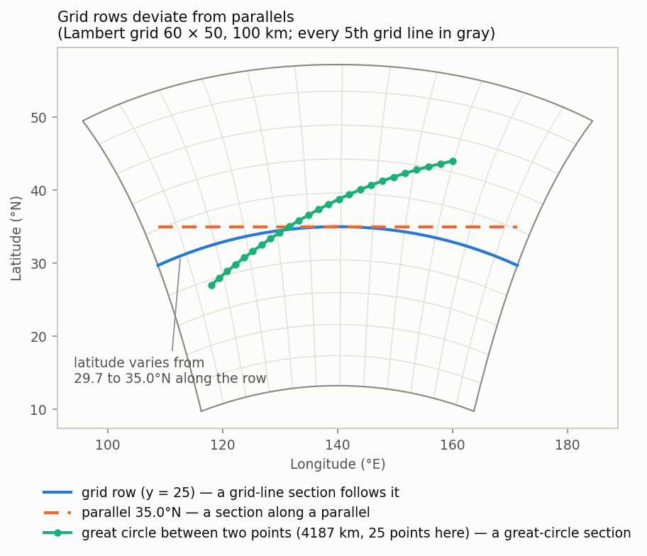
To draw a section along a parallel or between any two points, you need to find, for each point on the path, where that point lies in the grid, and interpolate from the surrounding grid-point values. On a grid with 1-D longitude/latitude the position is found in one dimension for each of the latitude and longitude axes, but on a 2-D coordinate grid the grid lines are curved, so the grid index has to be computed back from longitude/latitude. That inversion is the core of this chapter.
Overall flow — three stages
The interpolation proceeds in three stages, path points → fractional grid indices → values, and none of them uses any knowledge of the map projection. Everything is computed from the grid's longitude and latitude values (and the variable values) alone, so it works the same way for files without projection parameters and for grids in any projection.
| Stage | What it does | Function embedded in the reproduction script |
|---|---|---|
| 1. Take points on the path | For a parallel or meridian, divide the longitude (latitude) span evenly; for a great circle, take equally spaced points on the sphere | great_circle_points |
| 2. Express the point positions as grid indices | Express which cell each point falls in, and where within it, as fractional grid indices (fj, fi) | grid_fractional_indices (2-D) / grid_fractional_indices_1d (1-D) |
| 3. Interpolate from the four surrounding grid points | Weighted mean of the values at the four cell corners (bilinear interpolation) | sample_bilinear |
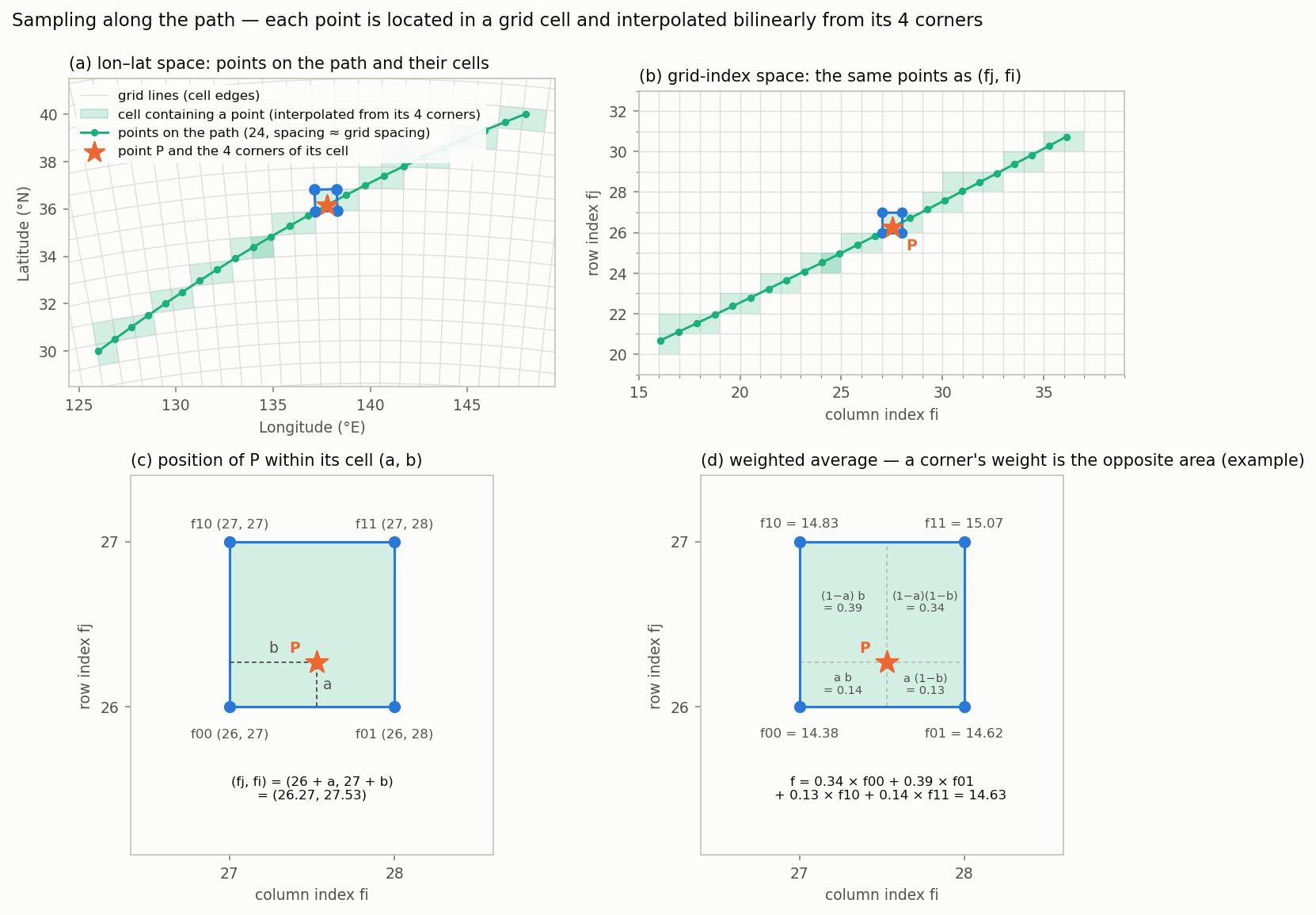
A fractional grid index extends the grid-point index (row j, column i) to a continuous quantity. If P in the figure has (fj, fi) = (26.27, 27.53), it lies in the cell spanning rows 26–27 and columns 27–28, at 0.27 along the row direction and 0.53 along the column direction (the integer part identifies the cell, the fractional part the position within it).
1. Taking points on the path
- Parallel (latitude fixed): the span between the start and end longitudes is divided evenly, and the latitude is a fixed value. The horizontal axis is longitude.
- Meridian (longitude fixed): the span between the start and end latitudes is divided evenly, and the longitude is a fixed value. The horizontal axis is latitude.
- Great circle between two points: the start and end points become unit vectors p1, p2 on the sphere, and equally spaced points are generated by spherical linear interpolation (slerp). The horizontal axis is the distance from the start (km).
- Because t is divided evenly between 0 and 1, the points are equally spaced along the great circle. ω is computed with atan2 so that precision holds both for two very close points and for two far-apart points (arccos loses precision when ω is near 0 or π).
- Longitude is made continuous along the path. Even across the dateline it runs 170 → 190 rather than jumping 179 → −179, so there is no jump when the path is drawn on a map or when longitude is the horizontal axis.
- If the start and end points are on opposite sides of the Earth (antipodal), the great circle is not unique, and an error is raised.
- The number of points is, by default, the path length divided by the grid spacing, rounded up, plus 1 (2–5000). The grid spacing is the median spherical distance between neighboring grid points on a 2-D coordinate grid, and the smaller of the latitude spacing and "longitude spacing × cos(latitude of the path)" on a 1-D grid. A 1000 km path on ClimCORE (5 km) gives about 200 points. Uncheck "Automatic number of points (spacing ≈ grid spacing)" to specify the number directly.
2. Expressing the point positions as grid indices
Grids with 2-D longitude/latitude
Using only the 2-D arrays of grid longitude and latitude, the fractional grid indices of each point are found in three steps. The figure shows the example of point P, whose true grid index, constructed from the projection, is (23.37, 31.62).

Step 1 — coarse nearest point on a thinned grid (a). When longitude and latitude are converted to 3-D unit vectors on the sphere, the spherical distance between two points is shorter the larger their dot product. So the dot products between P and the grid points thinned in both rows and columns (thinning stride = the number of points along the longer side of the grid ÷ 100, rounded up) are taken, and the largest gives the coarse nearest point. For ClimCORE (817 × 661) the stride is 9, so dot products with only 91 × 74 = 6,734 points are needed. Because the comparison is made with 3-D vectors, it is unaffected by the longitude convention (0–360 / −180–180), the dateline, or the poles.
Step 2 — moving the window to the true nearest grid point (b). Dot products are taken with all grid points in a window of one stride around the coarse nearest point (center ± stride). If the nearest point in the window differs from the center, the window is moved there and the search repeats; once the center is the nearest point in the window, it is final. In the figure the window moves once, from the coarse nearest point (25, 30) to the nearest grid point (23, 32), and stops.
Step 3 — Newton's method on the plane tangent at P (c, d). The grid points around the nearest grid point are projected gnomonically onto the plane tangent to the sphere at P. A unit vector v maps as follows, where p is the unit vector of P and e, n are the eastward and northward unit vectors at P. On this plane P is at the origin.
A square cell in grid-index space (c) becomes a quadrilateral on the plane (d). From the plane coordinates of the four cell corners x00, x01, x10, x11 (and likewise for y), consider the bilinear map that sends the position (a, b) within the cell (a along rows, b along columns, both 0–1) to a point on the plane, and solve for the (a, b) at which X = Y = 0 (the position of P) by Newton's method.
- The 2 × 2 Jacobian ∂(X, Y)/∂(a, b) can be written analytically from the corner coordinates. The iteration starts at the nearest grid point (a = b = 0); each update is limited to one cell in each direction, and the current cell is re-selected after every update, so the iteration can move on even when P lies in a neighboring cell. It stops after at most 8 iterations, or as soon as the update is less than 1e-10. The solution is the grid index (fj, fi) = (cell row + a, cell column + b).
- Why solve on the tangent plane: solving in the longitude–latitude plane would need separate handling of the longitude jump at the dateline, the singularity of longitude at the poles, and the distortion at high latitudes. On the tangent plane the distortion near P is small, and the eastward and northward unit vectors are defined even at the poles. Great circles are straight lines in the gnomonic projection, so the cell edges are also nearly straight on the plane.
- Points outside the grid or not converging: if the residual after solving (the offset from P on the plane) exceeds 1e-6 of the cell size, the point is treated as not converged and set to missing. Points whose grid index falls outside the grid range (0 to number of rows − 1, 0 to number of columns − 1) are outside the grid and are missing (points exactly on the boundary count as inside). If every point on the path is outside the grid, an error is raised; if only some are, those points stay missing and the edge of the figure is left blank.
- Accuracy: a true grid that is equally spaced in the projection plane is not exactly bilinear on the tangent plane, so a small error remains. The error shrinks in proportion to the cell size: measured values are 8e-4 cells for a 100 km grid and 3e-5 cells (about 15 cm) for a 5 km grid (the same as ClimCORE).
- Speed: on the ClimCORE grid, the grid indices of a 260-point path take 0.02 seconds.
Grids with 1-D longitude/latitude
On an ordinary grid with 1-D longitude/latitude, the index is found independently for each of the latitude and longitude axes. The coordinate values are sorted in ascending order, the index corresponding to the point's value is interpolated linearly (numpy's interp), and values outside the range are set to missing.
- Ascending and descending: the indices refer to the original order, so latitude running from north to south (90 → −90) and the like are handled as they are.
- Longitude convention: the point's longitude is moved by modulo into the 360° range starting at the grid's minimum longitude (on a 0–357.5° grid, −1° is treated as 359°).
- Seam of a global grid: if "last longitude − first longitude + grid spacing = 360°", the grid is treated as wrapping around in longitude, and the first column (+360°) is appended after the last column for the interpolation. Points crossing the seam (such as 359° on a 0–357.5° grid) are interpolated between the last and first columns.
| Grid | Point | Column index fi |
|---|---|---|
| 0–357.5°, 2.5° spacing (144 columns) | 10° | 4.0 |
| Same | −1° (= 359°) | 143.6 (between the 357.5° column and the 0° column) |
| Regional grid 100–160° | −200° (= 160°) | 24.0 (eastern edge) |
| Same | 170° | missing (outside the region) |
Expanding to a 2-D grid and using the method above gives almost the same indices (a difference of 2.7e-3 cells on a 2.5° grid). Because they do not agree exactly, the 1-D method is used for ordinary grids.
3. Bilinear interpolation from the four surrounding grid points
The value at the fractional grid index (fj, fi) = (j0 + a, i0 + b) is a weighted mean of the values at the four cell corners. f00 is the value at corner (j0, i0), f01 at (j0, i0 + 1), f10 at (j0 + 1, i0), and f11 at (j0 + 1, i0 + 1).
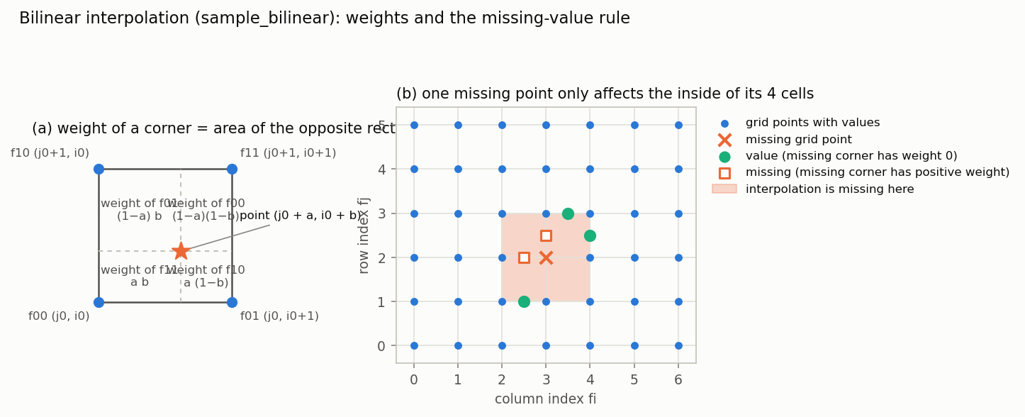
The weight of each corner equals the area of the rectangle on the opposite side of the point (figure a below). If the point coincides with a corner, the result is that corner's value itself; if it lies on a cell edge, it is the linear interpolation of the values at the two ends of the edge.
- Vertical, time and other dimensions are untouched: only the two horizontal dimensions are replaced by the one path dimension (e.g. (lev, y, x) → (lev, path)). There is no interpolation in the vertical or in time.
- Missing-value rule: if any corner with positive weight is missing, the point is missing. Missing corners with zero weight have no effect. This avoids fabricating values where data are missing below the ground or near land in ocean data, while a point exactly on a grid point is not wiped out by a missing neighbor.
- Outside the grid: points whose grid index is missing (outside the grid) give a missing result.
- Seam of a global grid: on a global grid with 1-D longitude/latitude, the first column is used as the column after the last, so the interpolation crosses the seam.
- Terrain mask: when the terrain mask is used with a section along a path, surface pressure or terrain height is mapped onto the path with the same bilinear interpolation before the ground is determined.
Limits and notes
- Seam of a periodic 2-D coordinate grid: on a global 2-D coordinate grid that wraps around in longitude (such as an ocean tripolar grid), points falling in the cell between the last and first columns are missing (treated as outside the grid). A global grid with 1-D longitude/latitude can interpolate across the seam.
- Near grid points with missing longitude/latitude: points in a cell that has a grid point with missing longitude/latitude as a corner are missing. When Newton's method started from the nearest grid point passes through such a cell, a point in a neighboring normal cell may also become missing (the choice errs on the side of not producing values).
- Vector and streamline components: in a great-circle section, vector and streamline components are interpolated and drawn as the chosen variables, without projection onto the section direction (a note appears in the box).
- Horizontal-axis range and averaging: in a section along a path, the horizontal-axis range is determined by the path, and horizontal range means are not available. The vertical range and the fixing or averaging of other dimensions such as time work as before.
Checking in the reproduction script
The functions used for the interpolation are embedded verbatim at the top of the reproduction script (only those used: great_circle_points for a great circle, grid_fractional_indices for a 2-D coordinate grid, grid_fractional_indices_1d for a 1-D grid, always sample_bilinear for a section along a path, and lonlat_tick_label when longitude/latitude are shown alongside the ticks). The in-app drawing and the reproduction script interpolate with literally the same code, so the figures match, and the script runs with numpy and xarray alone. For a great-circle section on a 2-D coordinate grid, the relevant part looks like this.
The start and end points and the number of points are written as literals, so you can move the section by editing them in the script. Reading the function bodies lets you follow the steps of this chapter directly.
What the tests verify
The ClimCanvas tests check the following about this interpolation automatically (tests/test_section_path.py and others).
- Great-circle points: the endpoints match, the distance agrees with the haversine formula, the points are equally spaced, and all points lie on the plane of the great circle. Longitude is continuous across the dateline. Paths through the pole, start = end, and the antipodal error.
- 2-D grid indices: the true grid indices constructed with a cartopy projection are recovered (tolerance 2e-3 cells on a 100 km grid, 1e-4 cells on a 5 km grid). Because the function itself does not use the projection, this is an independent check. A grid crossing the 180° seam, the pole itself on a polar stereographic grid, points outside the grid, and missing longitude/latitude.
- 1-D grid indices: global grids (descending latitude, longitude conventions, the seam), descending longitude, and points outside a regional grid. Agreement between the 1-D and 2-D methods.
- Bilinear interpolation: a bilinear field (2 + 3j − i + 0.5ij) is reproduced exactly. Missing corners with zero weight are ignored, and missing corners with positive weight give missing. Interpolation across the global seam.
- Section drawing: the drawn array of a section along a parallel matches values computed back analytically on a grid whose longitude/latitude are linear in the grid indices. The in-app figure and the reproduction-script figure match pixel for pixel.
- Real data: with ClimCORE Z (817 × 661, 17 pressure levels), sections along a parallel, a meridian, a great circle and a grid row matched pixel for pixel between the app and the reproduction script (about 2 seconds per section).